1 Q-learning

In Reinforcement Learning we are interested in maximizing the Expected Return so we usually work directly with those expectations. For instance, in Q-learning with function approximation we want to minimize the error \[\begin{align*}\mathbb{E}_{s,a}\left[\left(r(s,a)+\gamma\mathbb{E}_{s'}\left[\max_{a'}Q(s',a')\right]-Q(s,a)\right)^{2}\right],\end{align*}\] or, equivalently, \[\begin{align} \mathbb{E}_{s,a,s'}\left[\left(r(s,a)+\gamma\max_{a'}Q(s',a')-Q(s,a)\right)^{2}\right],\label{eq:classic_td_error} \end{align}\] where \(r(s,a)\) is the expected immediate reward. In semi-gradient methods we do this by moving \(Q(s,a)\) towards the target \(r(s,a)+\gamma\max_{a'}Q(s',a')\), pretending that the target is constant, and in DQN(Mnih et al. 2015) we even freeze the “target network” to improve stability even further.

The main idea of Distributional RL(M. G. Bellemare, Dabney, and Munos 2017) is to work directly with the full distribution of the return rather than with its expectation. Let the random variable \(Z(s,a)\) be the return obtained by starting from state \(s\), performing action \(a\) and then following the current policy. Then \[\begin{align*}Q(s,a)=\mathbb{E}[Z(s,a)].\end{align*}\] Instead of trying to minimize the error \(\ref{eq:classic_td_error}\), which is basically a distance between expectations, we can instead try to minimize a distributional error, which is a distance between full distributions: \[\begin{align} \sup_{s,a}\mathrm{dist}\left(R(s,a)+\gamma Z(s',a^{*}),Z(s,a)\right)\label{eq:distrib_td_error}\\ s'\sim p(\cdot|s,a)\nonumber \end{align}\] where you can mentally replace \(\sup\) with \(\max\), \(R(s,a)\) is the random variable for the immediate reward, and \[\begin{align*}a^{*}=\underset{a'}{\mathrm{arg\,max}\,}Q(s',a')=\underset{a'}{\mathrm{arg\,max}\,}\mathbb{E}[Z(s',a')].\end{align*}\] Note that we’re still using \(Q(s,a)\), i.e. the expected return, to decide which action to pick, but we’re trying to optimize distributions rather than expectations (of those distributions).

There’s a subtlety in expression \(\ref{eq:distrib_td_error}\): if \(s,a\) are constant, \(Z(s,a)\) is a random variable, but even more so when \(s\) or \(a\) are themselves random variables!

2 Policy Evaluation

Let’s consider policy evaluation for a moment. In this case we want to minimize \[\begin{align*}\mathbb{E}_{s,a,s',a'}\left[\left(r(s,a)+\gamma Q(s',a')-Q(s,a)\right)^{2}\right]\end{align*}\] We can define the Bellman operator for evaluation as follows: \[\begin{align*}(\mathcal{T}^{\pi}Q)(s,a)=\mathbb{E}_{s'\sim p(\cdot|s,a),a'\sim\pi(\cdot|s')}[r(s,a)+\gamma Q(s',a')]\end{align*}\] The Bellman operator \(\mathcal{T}^{\pi}\) is a \(\gamma\)-contraction, meaning that \[\begin{align*}\mathrm{dist}\left(\mathcal{T}Q_{1},\mathcal{T}Q_{2}\right)\leq\gamma\mathrm{dist}\left(Q_{1},Q_{2}\right),\end{align*}\] so, since \(Q^{\pi}\) is a unique fixed point (i.e. \(\mathcal{T}Q=Q\iff Q=Q^{\pi}\)), we must have that \(\mathcal{T}^{\infty}Q=Q^{\pi}\), disregarding approximation errors.

It turns out (M. G. Bellemare, Dabney, and Munos 2017) that this result can be ported to the distributional setting. Let’s define the Bellman distribution operator for evaluation in an analogous way: \[\begin{align*} (\mathcal{T}_{D}^{\pi}Z)(s,a) & =R(s,a)+\gamma Z(s',a')\\ s' & \sim p(\cdot|s,a)\\ a' & \sim\pi(\cdot|s') \end{align*}\] \(\mathcal{T}_{D}^{\pi}\) is a \(\gamma\)-contraction in the Wasserstein distance \(\mathcal{W}\), i.e. \[\begin{align*}\sup_{s,a}\mathcal{W}\left(\mathcal{T}_{D}^{\pi}Z_{1}(s,a),\mathcal{T}_{D}^{\pi}Z_{2}(s,a)\right)\leq\gamma\sup_{s,a}\mathcal{W}(Z_{1}(s,a),Z_{2}(s,a))\end{align*}\] This isn’t true for the KL divergence.

Unfortunately, this result doesn’t hold for the control (the one with the \(\max\)) version of the distributional operator.

3 KL divergence

3.1 Definition

I warn you that this subsection is highly informal.

If \(p\) and \(q\) are two distributions with same support (i.e. their pdfs are non-zero at the same points), then their KL divergence is defined as follows: \[\begin{align*}\mathrm{KL}(p\|q)=\int p(x)\log\frac{p(x)}{q(x)}dx.\end{align*}\]

Let’s consider the discrete case: \[\begin{align*}\mathrm{KL}(p\|q)=\sum_{i=1}^{N}p(x_{i})\log\frac{p(x_{i})}{q(x_{i})}=\sum_{i=1}^{N}p(x_{i})[\log p(x_{i})-\log q(x_{i})].\end{align*}\] As we can see, we’re basically comparing the scores at the points \(x_{1},\ldots,x_{N}\), weighting each comparison according to \(p(x_{i})\). Note that the KL doesn’t make use of the values \(x_{i}\) directly: only their probabilities are used! Moreover, if \(p\) and \(q\) have different supports, the KL is undefined.

3.2 How to use it

Now say we’re using DQN and extract \((s,a,r,s')\) from the replay buffer. A “sample of the target distribution” is \(r+\gamma Z(s',a^{*})\), where \(a^{*}=\mathrm{arg\,max}_{a'}Q(s',a')\). We want to move \(Z(s,a)\) towards this target (by keeping the target fixed).

I called \(r+\gamma Z(s',a^{*})\) a “sample of a distribution”, but the correct way to say it is that \(r+\gamma Z(s',a^{*})\) is a collection of samples of the real target distribution. The target distribution we want to learn is \(r+\gamma Z(s',a^{*})\) where \(r\) and \(s'\) are random variables. Since we sampled \(r\) and \(s'\), then the atoms of \(r+\gamma Z(s',a^{*})\) are just samples from the real target distribution and not a representation in atom form of that distribution. Indeed, to get a single sample from the real target distribution, we should first sample \(r\) and \(s'\), and, finally, sample from the distribution \(r+\gamma Z(s',a^{*})\). This is almost exactly what we’re doing since \(r\) and \(s'\) extracted from the replay buffer were indeed sampled. The only difference is that instead of sampling from \(r+\gamma Z(s',a^{*})\), we use all its atoms.

Let’s say we have a net which models \(Z\) by taking a state \(s\) and returning a distribution \(Z(s,a)\) for each action. For instance, we can represent each distribution through a softmax like we often do in Deep Learning for classification tasks. In particular, let’s choose some fixed values \(x_{1},\ldots,x_{N}\) for the support of all the distributions returned by the net. To simplify things, let’s make them equidistant so that \[\begin{align*}x_{i+1}-x_{i}=d=(x_{N}-x_{1})/(N-1),\qquad i=1,\ldots,N-1\end{align*}\] The pmf looks like a comb:

Since the values \(x_{1},\ldots,x_{N}\) are fixed, we just have to return \(N\) probabilities for each \(Z(s,a)\), so the net takes a single state and returns \(|\mathcal{A}|N\) scalars, where \(|\mathcal{A}|\) is the number of possible actions.

If \(p_{1},\ldots,p_{N}\) and \(q_{1},\ldots,q_{N}\) are the probabilities of the two distributions \(p\) and \(q\), then their KL is simply \[\begin{align*}\mathrm{KL}(p\|q)=\sum_{i=1}^{N}p_{i}\log\frac{p_{i}}{q_{i}}=H(p,q)-H(p)\end{align*}\] and if you’re optimizing wrt \(q\) (i.e. you’re moving \(q\) towards \(p\)), then you can drop the entropy term.

Also, we can recover \(Q(s,a)\) very easily: \[\begin{align*}Q(s,a)=\mathbb{E}[Z(s,a)]=\sum_{i=1}^{N}p_{i}x_{i}.\end{align*}\]

The interesting part is the transformation. In distributional Q-learning we want to move \(Z(s,a)\) towards \(r+\gamma Z(s',a^{*})\), but how do we put \(p\) in “standard comb form”? This is the projection part described in (M. G. Bellemare, Dabney, and Munos 2017) and it’s very easy. To form the target distribution we start from \(p=Z(s',a^{*})\), which is already in the standard form \(p_{1},\ldots,p_{N}\) and we look at the pairs \((x_{1},p_{1}),\ldots,(x_{N},p_{N})\) as if they represented samples with weights, which the authors of (M. G. Bellemare, Dabney, and Munos 2017) call atoms. This means that we can transform the distribution \(p\) just by transforming the position of its atoms. The transformed atoms corresponding to \(r+\gamma Z(s',a^{*})\) are \[\begin{align*}(r+\gamma x_{1},p_{1}),(r+\gamma x_{2},p_{2}),\ldots,(r+\gamma x_{N},p_{N}).\end{align*}\] Note that the weights \(p_{i}\) don’t change. The problem is that now we have atoms which aren’t in the standard positions \(x_{1},\ldots,x_{N}\). The solution proposed in (M. G. Bellemare, Dabney, and Munos 2017) is to split each misaligned atom into the two closest aligned atoms by making sure to distribute its weight according to its distance from the two misaligned atoms:

Observe the proportions very carefully. Let’s say the green atom has weight \(w.\) For some constants \(c\), the green atom is at distance \(3c\) from \(x_{6}\) and \(c\) from \(x_{7}\). Indeed, the atom at \(x_{6}\) receives weight \(\frac{1}{4}w\) and the atom at \(x_{7}\) weight \(\frac{3}{4}w\), which makes sense. Also, note that the probability mass is conserved so there’s no need to normalize after the splitting. Of course, since we need to split all the transformed atoms, individual aligned atoms can receive contributions from different atoms. We simply sum all the contributions. This is how the authors do it, but it’s certainly not the only way.

3.3 The full algorithm

Here’s the algorithm taken directly (cut & pasted) from (M. G. Bellemare, Dabney, and Munos 2017):

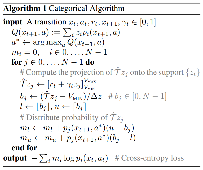
Assume we’ve just picked \((x_{t},a_{t},r_{t},x_{t+1})\) from the replay buffer in some variant of the DQN algorithm, so \(x\) is used to indicate states. The \(z_{0},\ldots,z_{N-1}\) are the fixed global positions of the atoms (i.e. our \(x_{1},\ldots,x_{N}\) in figure 2). Let’s assume there’s just a global \(\gamma\).

Let’s go through the algorithm in detail assuming we’re using a neural network for \(Z\):

1. We feed \(x_{t+1}\) to our net which outputs an \(|\mathcal{A}|\times N\) matrix \(M(x_{t+1})\), i.e. each row corresponds to a single action and contains the probabilities for the \(N\) atoms. That is, the row for action \(a\) contains the vector \[\begin{align*}(p_{0}(x_{t+1},a),\ldots,p_{N-1}(x_{t+1},a))\end{align*}\]

2. We compute all the \[\begin{align*}Q(x_{t+1},a)=\mathbb{E}\left[Z(x_{t+1},a)\right]=\sum_{i=0}^{N-1}z_{i}p_{i}(x_{t+1},a)\end{align*}\] as follows: \[\begin{align*}Q(x_{t+1})=M(x_{t+1})\begin{bmatrix}z_{0}\\ z_{1}\\ \vdots\\ z_{N-1} \end{bmatrix}.\end{align*}\] Note that \(Q(x_{t+1})\) is a column vector of length \(|\mathcal{A}|\).

3. Now we can determine the optimum action \[\begin{align*}a^{*}=\mathrm{arg\,max_{a}}Q(x_{t+1},a)\end{align*}\] Let \(q=(q_{0},\ldots,q_{N-1})\) be the row of \(M(x_{t+1})\) corresponding to \(a^{*}\).

4. \(m_{0},\ldots,m_{N-1}\) will accumulate the probabilities of the aligned atoms of the target distribution \(r_{t}+\gamma Z(x_{t+1},a^{*})\). We start by zeroing them.

5. The non-aligned atoms of the target distribution are at positions \[\begin{align*}\hat{\mathcal{T}}z_{j}=r_{t}+\gamma z_{j},\qquad j=0,\ldots,N-1\end{align*}\] We clip those positions so that they are in \([V_{\mathrm{MIN}},V_{\mathrm{MAX}}]\), i.e. \([z_{0},z_{N-1}]\).

6. Assuming that the adjacent aligned atoms are at distance \(\Delta z\), the indices of the closest aligned atoms on the left and on the right of \(\hat{\mathcal{T}}z_{j}\) are, respectively: \[\begin{align*} l & =\left\lfloor \frac{\hat{\mathcal{T}}z_{j}-z_{0}}{\Delta z}\right\rfloor \\ u & =\left\lceil \frac{\hat{\mathcal{T}}z_{j}-z_{0}}{\Delta z}\right\rceil \end{align*}\]

7. Now we need to split the weight of \(\hat{\mathcal{T}}z_{j}\), which is \(q_{j}\), between \(m_{l}\) and \(m_{r}\) as we saw before. Note that \[\begin{align*} (u)-(b_{j}) & =\left(\frac{z_{u}-z_{0}}{\Delta z}\right)-\left(\frac{\hat{\mathcal{T}}z_{j}-z_{0}}{\Delta z}\right)=\frac{z_{u}-\hat{\mathcal{T}}z_{j}}{z_{u}-z_{l}}\\ (b_{j})-(l) & =\left(\frac{\hat{\mathcal{T}}z_{j}-z_{0}}{\Delta z}\right)-\left(\frac{z_{l}-z_{0}}{\Delta z}\right)=\frac{\hat{\mathcal{T}}z_{j}-z_{l}}{z_{u}-z_{l}} \end{align*}\] which means that, as we said before, the weight \(q_{j}\) is split between \(z_{l}\) and \(z_{u}\) (indeed, \(u-b_{j}+b_{j}-l=1)\), and the contribution to \(m_{l}\) is proportional to the distance of \(\hat{\mathcal{T}}z_{j}\) from \(z_{u}\). The more distant it is from \(z_{u}\), the higher the contribution to \(m_{l}\).

8. Now we have the probabilities \(m_{0},\ldots,m_{N-1}\) of the aligned atoms of \(r_{t}+\gamma Z(x_{t+1},a^{*})\) and, of course, the probabilities \[\begin{align*}p_{0}(x_{t},a_{t};\theta),\ldots,p_{N-1}(x_{t},a_{t};\theta)\end{align*}\] of the aligned atoms of \(Z(x_{t},a)\), which are the ones we want to update. Thus \[\begin{align*} \nabla_{\theta}\mathrm{KL}(m\|p_{\theta}) & =\nabla_{\theta}\sum_{i=0}^{N-1}m_{i}\log\frac{m_{i}}{p_{\theta}}\\ & =\nabla_{\theta}\left[H(m,p_{\theta})-H(m)\right]\\ & =\nabla_{\theta}H(m,p_{\theta}) \end{align*}\] That is, we can just use the cross-entropy \[\begin{align*}H(m,p_{\theta})=-\sum_{i=0}^{N-1}m_{i}\log p_{i}(x_{t},a_{t};\theta)\end{align*}\] for the loss.

4 Wasserstein distance

The first paper (M. G. Bellemare, Dabney, and Munos 2017) about distributional RL left a gap between theory and practice because the theory requires the Wasserstein distance, but in practice they used a KL-based procedure.

The second paper (Dabney et al. 2017) closes the gap in a very elegant way.

4.1 A different idea

This time I won’t start with a definition, but with an idea. Rather than use atoms with fixed positions, but variable weights, let’s do the opposite: let’s use atoms with fixed weights, but variable positions. Moreover, let’s use the same weight for each atom, i.e. \(1/N\) if the atoms are \(N\).

But how do we represent distributions this way? It’s very simple, really. We slice up the distribution we want to represent into \(N\) slices of \(1/N\) mass and put each atom at the median of a slice. This makes sense; in fact, the atoms weigh \(1/N\) as well:

If the atoms are \(N\) then the \(i\)-th atom corresponds to a quantile of \[\begin{align*}\hat{\tau}_{i}=\frac{2(i-1)+1}{2N},\qquad i=1,\ldots,N\end{align*}\] as shown in the following picture:

4.2 How do we determine a quantile?

4.2.1 Determining the median

The median is just the \(0.5\) quantile, i.e. a point which has \(0.5\) mass on the left and \(0.5\) mass on the right. In other words, it splits the probability mass in half. So let’s say we have a random variable \(X\) and we know how to draw samples. How can we compute the median? We start with a guess \(\theta\), draw some samples and if \(\theta\) has more samples on the left than on the right, we move it a little to the left. By symmetry, we move it to the right if it has more samples on the right. Then we repeat the process and keep updating \(\theta\) until convergence.

We should move \(\theta\) in proportion to the disparity between the two sides, so let’s decide that each sample on the left subtract \(\alpha\) and each sample on the right add \(\alpha\). Basically, \(\alpha\) is a learning rate. If it’s too small the algorithm takes too long and if it’s too big the algorithm fluctuates a lot around the optimal solution. Here’s a picture about this method:

We reach the equilibrium when \(\theta\) is the median. Doesn’t this look like SGD with a minibatch of \(16\) samples and learning rate \(\alpha\)? What’s the corresponding loss? The loss is clearly \[\begin{align}L_{\theta}=\mathbb{E}_{X}[|X-\theta|]\label{eq:median_loss}\end{align}\] This should look familiar to any statistician. Note that in the picture above we’re adding the gradients, but when we minimize we subtract them so gradients on the left of \(\theta\) must be \(1\) and on the right \(-1\): \[\begin{align*}\nabla_{\theta}L_{\theta}=\begin{cases} \nabla_{\theta}(\theta-X)=1 & \text{if }X<\theta\\ \nabla_{\theta}(X-\theta)=-1 & \text{if }X\geq\theta \end{cases}\end{align*}\]

4.2.2 Determining any quantile

We can generalize this to any quantile by using different weights for the left and right samples. Let’s omit the \(\alpha\) for more clarity, since we know it’s just the learning rate by now. If we want the probability mass on the left of \(\theta\) to be \(\tau\), we need to use weight \(1-\tau\) for the samples on the left and \(\tau\) for the ones on the right. This works because, when \(\theta\) is the \(\tau\) quantile, if we sample \(S\) samples then, on average, the samples on the left will be \(\tau S\) and the ones on the right \((1-\tau)S\). Multiplying the number of samples by their weights, we get an equality: \[\begin{align*}(\tau S)(1-\tau)=((1-\tau)S)(\tau)\end{align*}\] so both sides pull with equal strength if and only if \(\theta\) is the \(\tau\) quantile.

Basically, we need to scale the weights/gradients on the left of \(\theta\) by \(1-\tau\) and the ones on the right by \(\tau\), which are both nonnegative scalars, since \(\tau\in[0,1]\). Here’s a compact expression for that: \[\begin{align*}|\tau-\delta_{X<\theta}|=\begin{cases} |\tau-1|=1-\tau & \text{if }X<\theta\\ \tau & \text{if }X\geq\theta \end{cases}\end{align*}\] Therefore, we just need to multiply the \(|X-\theta|\) in the loss \(\ref{eq:median_loss}\) by \(|\tau-\delta_{X<\theta}|\): \[\begin{align*} L_{\theta} & =\mathbb{E}_{X}[|X-\theta||\tau-\delta_{X<\theta}|]\\ & =\mathbb{E}_{X}[\rho_{\tau}(X-\theta)] \end{align*}\] where \[\begin{align} \rho_{\tau}(u) & =|u||\tau-\delta_{u<0}|\label{eq:rho_t_abs}\\ & =u(\tau-\delta_{u<0})\label{eq:rho_t_no_abs} \end{align}\] Note that we can eliminate the two absolute values because the two factors have always the same sign. Expression \(\ref{eq:rho_t_no_abs}\) is the one we find in equation (8) in (Dabney et al. 2017), but expression \(\ref{eq:rho_t_abs}\) makes it clearer that we can eliminate the cuspid in \(\rho_{t}\) by replacing \(|u|\) with the Huber loss defined as: \[\begin{align*}\mathcal{L}_{\kappa}(u)=\begin{cases} \frac{1}{2}u^{2} & \text{if }|u|\leq\kappa\\ \kappa(|u|-\frac{1}{2}\kappa) & \text{otherwise } \end{cases}\end{align*}\] This makes optimization easier, according to the authors of (Dabney et al. 2017). We’re interested in \(\mathcal{L}_{1}\) in particular because it’s the only one with the right slopes in the linear parts. Here’s a picture of the two curves:

Now we can define \(\rho_{\kappa}\) as follows: \[\begin{align*} \rho_{\tau}^{0}(u) & =\rho_{\tau}(u)=u(\tau-\delta_{u<0})\\ \rho_{\tau}^{\kappa}(u) & =\mathcal{L}_{\kappa}(u)|\tau-\delta_{u<0}| \end{align*}\]

Here’s a picture of \(\rho_{0.3}\) and \(\rho_{0.3}^{1}\):

The final loss becomes \[\begin{align*}L_{\theta}=\mathbb{E}_{X}[\rho_{\tau}^{1}(X-\theta)]\end{align*}\]

4.2.3 Computing all the needed quantiles at once

To compute more quantiles at once, we can just compute the total loss given by \[\begin{align*}L_{\theta}=\sum_{i=1}^{N}\mathbb{E}_{X}[\rho_{\tau_{i}}^{1}(X-\theta_{i})]\end{align*}\] where \(\theta=(\theta_{1},\ldots,\theta_{N})\) and we want \(\theta_{i}\) to be the \(\tau_{i}\) quantile. Of course, in general we can write \[\begin{align}L_{\theta}=\sum_{i=1}^{N}\mathbb{E}_{X}[\rho_{\tau_{i}}^{1}(X-f(\theta)_{i}]\label{eq:q_reg_formula}\end{align}\] where \(f\) is some \(\mathbb{R}^{N}\)-valued function of \(\theta\).

4.2.4 Some code

Here’s the code for drawing picture 4 in subsection 4.1:

import tensorflow as tf
import matplotlib.pyplot as plt
import numpy as np


class Quantiles:
    def __init__(self, taus, tf_graph=None):
        self.taus = taus
        N = len(taus)

        graph = tf_graph or tf.get_default_graph()
        with graph.as_default():
            with tf.variable_scope('quantiles'):
                self.xs = tf.placeholder('float')
                self.theta = tf.get_variable('theta', shape=(N,))
                self.loss = sum(
                    tf.reduce_mean(self._rho_tau(self.xs - self.theta[i],
                                                 taus[i], kappa=0))
                    for i in range(N))
                self.train_step = tf.train.AdamOptimizer(0.05).minimize(
                    self.loss)

    @staticmethod
    def _HL(u, kappa):
        delta = tf.cast(abs(u) <= kappa, 'float')
        return delta * (u * u / 2) + (1 - delta) * (
                kappa * (abs(u) - kappa / 2))

    @staticmethod
    def _rho_tau(u, tau, kappa=1):
        delta = tf.cast(u < 0, 'float')
        if kappa == 0:
            return (tau - delta) * u
        else:
            return abs(tau - delta) * Quantiles._HL(u, kappa)

    def get_quantiles(self, samples, loops):
        with tf.Session() as sess:
            tf.global_variables_initializer().run()
            for _ in range(loops):
                loss, _ = sess.run([self.loss, self.train_step],
                                   {self.xs: samples})
            qs = sess.run(self.theta)
        return qs


class MixtureOfGaussians:
    def __init__(self, pis, mus, sigmas):
        self.pis = pis
        self.mus = mus
        self.sigmas = sigmas

    def draw_samples(self, n):
        samples = np.empty(n)
        for i in range(n):
            idx = np.random.multinomial(1, self.pis).argmax()
            samples[i] = np.random.normal(self.mus[idx], self.sigmas[idx])
        return samples

    def pdf(self, x):
        return np.sum(pi * np.exp(-0.5 * ((x - mu) / s) ** 2) /
                        (s * np.sqrt(2 * pi))
                      for pi, mu, s in zip(self.pis, self.mus, self.sigmas))


tf.reset_default_graph()

MoG = MixtureOfGaussians(pis=[1/3, 1/3, 1/3], mus=[-3, 0, 5], sigmas=[2, 1, 2])
xs = np.linspace(-11, 11, num=200)
ys = MoG.pdf(xs)

N = 10  # num of quantiles
taus = [i / (2 * N) for i in range(0, 2 * N + 1)]
Q = Quantiles(taus)
samples = MoG.draw_samples(10000)
qs = Q.get_quantiles(samples, loops=2000)

plt.plot(xs, ys)

for q in qs[::2]:
    plt.plot([q, q], [0, MoG.pdf(q)], 'black')
plt.plot(qs[1::2], np.zeros_like(qs[1::2]), 'or')

plt.savefig('quantiles.svg', bbox_inches='tight')
plt.show()

4.3 Definition of the Wasserstein metric

Let \(X\) and \(Y\) be two scalar random variables and \(F_{X}\) and \(F_{Y}\) their CDFs. Then, their \(p\)-Wasserstein distance is \[\begin{align*}\mathcal{W}_{p}(X,Y)=\left(\int_{0}^{1}\left|F_{X}^{-1}(u)-F_{Y}^{-1}(u)\right|^{p}du\right)^{1/p}\end{align*}\] We’ll use the \(1\)-Wasserstein distance (i.e. with \(p=1\)) which measures the difference between the CDFs by measuring the area of a “discrepancy region” (the cyan region in the picture):

Now note that the CDF of a distribution represented by atoms \(y_{1},\ldots,y_{N}\) of probability mass \(q\) is a step function:

The cyan region, and thus the Wasserstein distance, is reduced when we slice up the red curve into \(q\)-mass slices and choose our atoms so that they halves the mass of each slice:

Note that in the picture above \[\begin{align*}\hat{\tau}_{i}=\frac{2(i-1)+1}{2N},\qquad i=1,\ldots,N\end{align*}\] with \(N=12\). The positions of our atoms are \[\begin{align*}y_{i}=F_{X}^{-1}(\hat{\tau}_{i}),\qquad i=1,\ldots,N\end{align*}\] where \(X\) is the variable associated with the red CDF.

Here’s what we get with \(30\) atoms:

So, it seems to be working!

4.4 The full algorithm

Here’s the full algorithm taken directly (cut & pasted) from (Dabney et al. 2017):

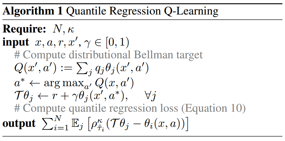
As before, let’s assume we’ve just picked \((x,a,r,x')\) from the replay buffer in some variant of the DQN algorithm, so \(x\) is used to indicate states. The algorithm is quite simple:

1. We recover \(Q(x')\) from \(Z(x')\) returned by our net. We can assume that \(q_{j}=\frac{1}{N}\), i.e. the atoms have the same weight.

2. We find \(a^{*}\) which is the optimal action according to \(Q(x'\)) (there’s a typo in the code).

3. Remember that the network, given a state (\(x'\) in this case), returns a matrix where each row contains the \(N\) atoms for a particular action. Let \(\theta'_{1},\ldots,\theta'_{N}\) be the atoms of \(Z(x',a^{*})\).

4. We treat the atoms \(\theta'_{1},\ldots,\theta'_{N}\) as samples and transform them directly: \[\begin{align*}\mathcal{T}\theta'_{j}=r+\gamma\theta'_{j},\qquad i=1,\ldots,N\end{align*}\]

5. Let \(\theta_{1},\ldots,\theta_{N}\) be the atoms of \(Z(x,a)\). We want to reduce the Wasserstein distance between \(Z(x,a)\) and \(r+\gamma Z(x',a^{*})\) by optimizing \(Z(x,a)\). As always, the target \(r+\gamma Z(x',a^{*})\) is treated as a constant for stability reasons (and we even use target freezing for extra stability).
   We have \(N\) samples for the target distribution, that is \(\mathcal{T}\theta'_{1},\ldots,\mathcal{T}\theta'_{j}\). So, we can use formula \(\ref{eq:q_reg_formula}\): \[\begin{align*}L_{\theta}=\sum_{i=1}^{N}\mathbb{E}_{X}\left[\rho_{\tau_{i}}^{1}(X-f(\theta)_{i})\right]\end{align*}\] In our case, the formula becomes \[\begin{align*} L_{\theta} & =\sum_{i=1}^{N}\mathbb{E}_{X}\left[\rho_{\tau_{i}}^{1}(X-f(\theta)_{i})\right]\\ & =\sum_{i=1}^{N}\mathbb{E}_{\mathcal{T}Z'}\left[\rho_{\hat{\tau}_{i}}^{1}(\mathcal{T}Z'-\theta_{i})\right],\qquad\mathcal{T}Z'=r+\gamma Z(x',a^{*})\\ & =\frac{1}{N}\sum_{i=1}^{N}\sum_{j=1}^{N}\left[\rho_{\hat{\tau}_{i}}^{1}(\mathcal{T}\theta'_{j}-\theta_{i})\right] \end{align*}\] where \[\begin{align*}\hat{\tau}_{i}=\frac{2(i-1)+1}{2N},\qquad i=1,\ldots,N\end{align*}\]

4.5 Why don’t we use simple regression?

Both the “moving” distribution and the target distribution are represented by \(N\) atoms each of weight \(1/N\):

So why don’t we avoid sampling and use simple regression? That is: \[\begin{align}L_{\theta}=\sum_{i=1}^{N}(\theta_{i}-\theta'_{i})^{2}\label{eq:simple_reg_loss}\end{align}\] The problem is that the atom positions \(\theta_{1},\ldots,\theta_{N}\) and \(\theta'_{1},\ldots,\theta'_{N}\) returned by the network are not guaranteed to be in any particular order, especially before convergence.

Note that the method described in subsection 4.4 doesn’t require that the atom positions be ordered from smaller to bigger. First, the target positions needn’t be sorted because they’re just used as samples. Second, the moving positions (i.e. the ones we want to update) can also be in any order because they’re trained “independently”: each atom will be moved towards the right position indicated by its corresponding \(\hat{\tau}_{i}\) irrespective of the positions and order of the other “moving” atoms.

I don’t know if this is a problem in the RL setting, but when I wrote the code to draw picture 4 (shown in subsection 4.2.4), I noticed that quantile regression requires many samples and quite a lot of training to get good results. In particular, since we’re using samples, the quality is especially low in intervals of low probability mass.

Moreover, note that, in the code, I used \(\rho_{\tau}^{0}\), the curve with the cuspid, and not \(\rho_{\tau}^{1}\), the smoothed out one, because I was getting worse results with the latter. Indeed, by replacing the “cuspid part” with a quadratic, we treat the samples which fall in the quadratic part as if we were computing the mean rather than the median.

One possible solution might be to return nonnegative distances between the points and then reconstruct the absolute positions of the atoms, which is very easy to do. This way we could use loss \(\ref{eq:simple_reg_loss}\) which is much more efficient.

4.5.1 A more fundamental reason

Will Dabney, one of the authors of the papers, pointed out that there’s a more fundamental reason why we can’t use simple regression: we might not find the correct quantiles!

I think Dabney tried to be tactful with his response, but the truth is that I didn’t think this through. I was focusing on getting faster convergence and forgot about what I wrote about \(r+\gamma Z(s',a^{*})\) being just a “sample” of the real distribution (link to relevant paragraph).

Let’s say we want to determine the median of the distribution \(r+\gamma Z(s',a^{*})\), where \(r\) and \(s'\) are both random variables. We focus on the median just for simplicity: this argument clearly applies to any quantiles.

We initialize the median of \(Z(s,a)\) to an initial guess \(\theta\) and then, at each step:

1. we get \(N\) samples of the real target distribution \(r+\gamma Z(s',a^{*})\),

2. we compute the median of the \(N\) samples we just received,

3. we use the median to update \(\theta\).

Basically, if \(m_{1},m_{2},\ldots\) is the sequence of medians, we end up computing \(\theta\) this way: \[\begin{align*}\hat{\theta}=\underset{\theta}{\mathrm{arg\,min}}\sum_{i}(m_{i}-\theta)^{2}\end{align*}\] This doesn’t give us the correct median because \[\begin{align*}\hat{\theta}=\sum_{i}m_{i}\end{align*}\] but the median of all the samples is not the mean of the medians. This is easy to see with a picture:

\(B_{1},B_{2},\ldots\) are the “batches” of \(N=5\) atoms and the medians \(m_{1},m_{2},\ldots\) are indicated by red circles. In this example, we keep receiving the same two batches (the blue and the green one) over and over. The correct solution is clearly \(\theta^{*}\) because it has half samples on the left and half on the right, but by using simple regression we get \(\theta^{\mathrm{wrong}}\), which, as you can see, is the mean of the medians.

And if we used the L1 loss instead? That is, \[\begin{align*}\hat{\theta}=\underset{\theta}{\mathrm{arg\,min}}\sum_{i}|m_{i}-\theta|\end{align*}\] This still wouldn’t work since the median of all the samples is not the median of the medians. The following picture should make that obvious:

If our initial guess is \(\theta^{\mathrm{wrong}}\) and the learning rate, \(\alpha\), is small enough, we won’t make any progress since we’ll keep adding \(\alpha\) and \(-\alpha\) to \(\theta\). Note that \(\theta^{\mathrm{wrong}}\) is indeed the median of the medians, but so is \(\theta^{*}\), according to the samples. Since no medians fall between \(\theta^{*}\) and \(\theta^{\mathrm{wrong}}\) in our example, the optimization algorithm can’t tell the two solutions apart.

Bibliography

Bellemare, Marc G., Will Dabney, and Rémi Munos. 2017. “A Distributional Perspective on Reinforcement Learning.” CoRR abs/1707.06887. http://arxiv.org/abs/1707.06887.
Dabney, W., M. Rowland, M. G. Bellemare, and R. Munos. 2017. “Distributional Reinforcement Learning with Quantile Regression.” ArXiv E-Prints, October.
Mnih, Volodymyr, Koray Kavukcuoglu, David Silver, Andrei A Rusu, Joel Veness, Marc G Bellemare, Alex Graves, et al. 2015. “Human-Level Control Through Deep Reinforcement Learning.” Nature 518 (7540). Nature Research:529–33.